To illustrate Bayesian DCA on survival data, we load the example
dataset dca_survival_data shown below.
library(bayesDCA)
head(dca_survival_data)
#>   outcomes.time outcomes.status model_predictions binary_test
#> 1     0.2948349       0.0000000        0.18806301           0
#> 2     1.8747960       0.0000000        0.25349061           1
#> 3     0.0355183       0.0000000        0.01025269           0
#> 4     1.2850960       0.0000000        0.04836840           0
#> 5     0.2398763       0.0000000        0.23502042           1
#> 6     2.0934150       0.0000000        0.04611183           0
The dataset contains the time-to-event outcomes (a
survival::Surv object), the predictions from a prognostic
model, and the results from a binary prognostic test. The time horizon
for the event prediction is one time units (e.g., year), so we set
prediction_time = 1. We also set chains = 1 to
speed up MCMC sampling with Stan (in
practice you should use at least chains = 4, maybe with
cores = 4 for speed as well).
Interrogating the output
We can do all kinds of output interrogation just like with binary outcomes.
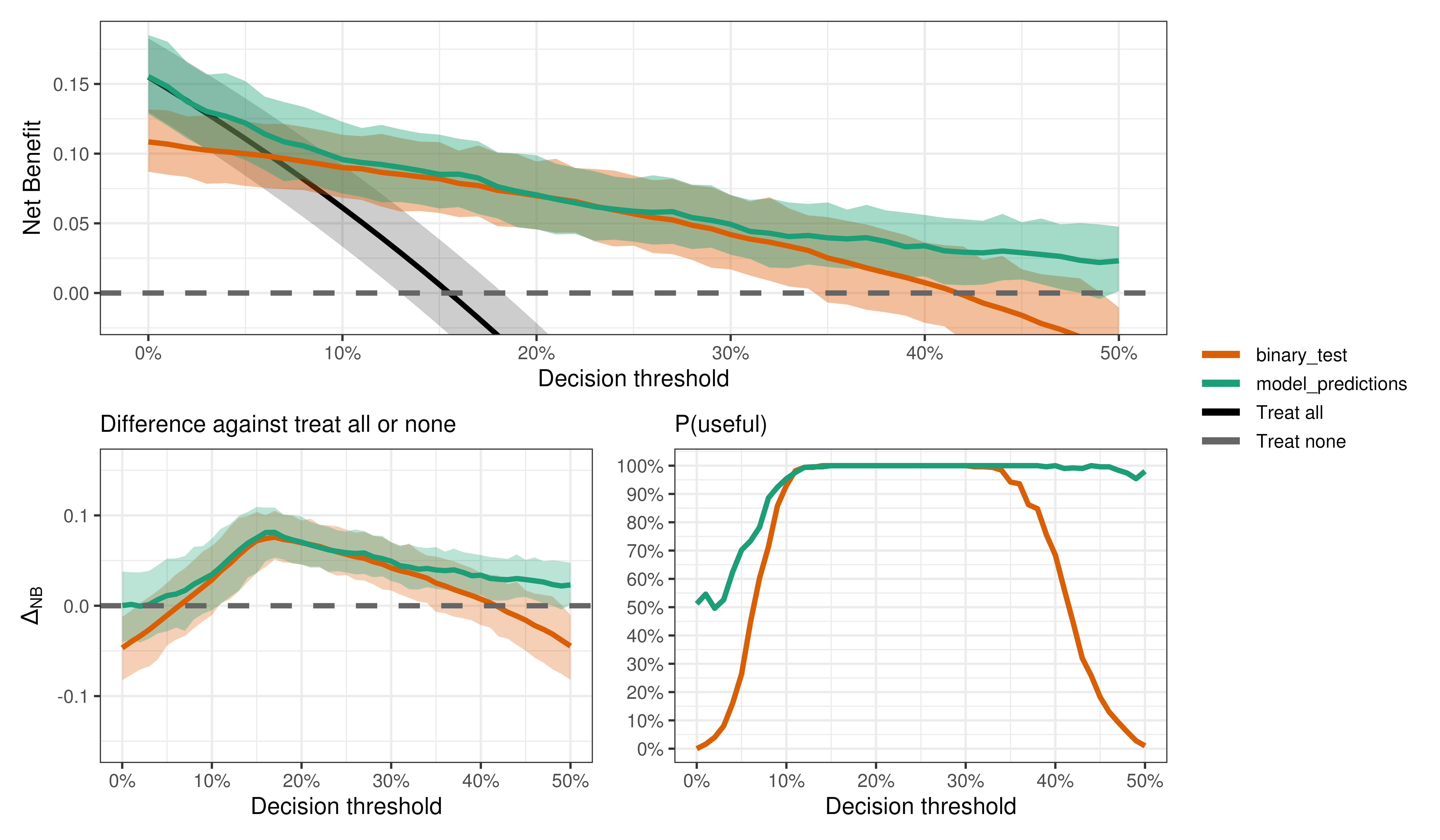
Is the model better than the test?
compare_dca(fit,
            strategies = c("model_predictions", "binary_test"),
            type = "pairwise")